Replication data for Mining biosynthetic gene clusters in Carnobacterium maltaromaticum by interference competition network and genome analysis
NOTE
Code used to analyse the data desribed in the manuscript Gontijo et al., 2022
path <- "/Users/borges5/Documents/TRAVAIL/R_wd/site_internet/content/post/network_genome_antimic/data-clean" # CHANGE ME TO YOUR PATH...
LIBRARIES
library(tidyverse)
library(ComplexHeatmap)
library(viridis)
library(ggrepel)
library(ggthemes)
library(ggprism)
library(factoextra)
DATA PREPARATION
Seed for reproducible code
set.seed(666)
Load the names of the strains described in (Ramia et al, 2020)
strains_ramia <- read.csv2(file.path(path,"strains_ramia2020.csv"),
                check.names = F,
                dec = ",",
                stringsAsFactors = T)
Load the graph data
mat <- read.csv2(file.path(path,"20220201_INHIB_MAT_ROW-SEND_clean2.csv"),
                check.names = F,
                dec = ",",
                stringsAsFactors = T)

names(mat)[1] <- "from"
load the table indicating which strains have been genome sequenced
genome <- read.csv2(file.path(path,"genome_bin.csv"),
                check.names = F,
                dec = ",",
                stringsAsFactors = T)

genome$genome <- as.character(genome$genome)
genome_yes <- genome %>%
  filter(genome==1)
genome_yes <- genome_yes$strain
genome_yes <- droplevels(genome_yes)
How many genomes were analyzed ?
length(genome_yes)
## [1] 29
Define the strains inhibiting EGDe by the kmeans clustering method
# make dataframe with the EGDe inhibition values
EGDe_inhib <- mat %>%
  select(from, EGDe) %>%
  column_to_rownames("from")
# Define the number of clusters
EGDe_inhib_sc <- scale(EGDe_inhib)
fviz_nbclust(EGDe_inhib_sc, kmeans, method = "silhouette")+
  labs(subtitle = "Silhouette method")

# => 2 clusters
# Kmeans clustering with the value of 2 clusters
km.out = kmeans(EGDe_inhib_sc,centers=2,nstart =20)
EGDe_inhib <-  data.frame(km.out$cluster)
EGDe_inhib <- rownames_to_column(EGDe_inhib, "from")
colnames(EGDe_inhib)[2] <- "EGDe_bin"
EGDe_inhib <- EGDe_inhib %>%
  mutate(EGDe_bin=ifelse(EGDe_bin==2, 1,0))
Build a binary matrix with all the data by using 300 as a threshold for Carno Vs Carno. For Carno Vs Listeria => use the EGDe_bin dataframe defined above
mat_bin <- mat

for (i in 2:77) {
  mat_bin[ , i]=ifelse(mat[ , i]>300, 1, 0)
}

mat_bin <- full_join(mat_bin,EGDe_inhib,by="from")


row.names(mat_bin) <- mat_bin$from
mat_bin <- select(mat_bin,-1)
Binary matrix without the values for Listeria
mat_df_bin <- select(mat_bin, 1:76)
Calculation of the degrees
# Degrees
## creation of an empty dataframe to store the results of calculation we'll do after
deg_receiver <- data.frame(strain=colnames(mat_df_bin),
                           Receiver=rep(0, ncol(mat_df_bin)))

deg_sender <- data.frame(strain=rownames(mat_df_bin),
                         Sender=rep(0, nrow(mat_df_bin)))


## Calculation of the Receiver degrees
for (i in 1:nrow(mat_df_bin)){
  deg_receiver[i, 2]<-sum(mat_df_bin[ ,i])
}

## Calculation of the Sender degrees
for (i in 1:ncol(mat_df_bin)){
  deg_sender[i, 2]<-sum(mat_df_bin[i,2:ncol(mat_df_bin)])
}
# Fusion matrix and degrees
deg <-  full_join(deg_sender, deg_receiver, by="strain")
deg_temp <- deg
names(deg_temp)[names(deg_temp)=="strain"] <- "from"
mat_inhib_deg <- full_join(mat,deg_temp, by="from")
rm(deg_temp)
# Create a column -+ for Listeria strainsn threshold 250.
mat_inhib_deg2 <- full_join(mat_inhib_deg,EGDe_inhib, by="from")
INHIBITION MATRIX
# Change the name of "strain" column to "from" in order to be able to make subsequent fusions with merge
names(deg_receiver)[names(deg_receiver)=="strain"] <- "from"
names(deg_sender)[names(deg_sender)=="strain"] <- "from"
# merge
send_ord <- mat %>%
  merge(deg_sender, on="from") %>%
  arrange(desc(Sender))

from <- send_ord$from

send_ord_sel <- select(send_ord, c(-1,-ncol(send_ord)))
colnames_send_ord <- names(send_ord_sel)
send_ord_sel_t <- t(send_ord_sel)
send_ord_sel_t <- as.data.frame(send_ord_sel_t)
names(send_ord_sel_t) <- from

send_ord_sel_t <- cbind(colnames_send_ord, send_ord_sel_t)

names(send_ord_sel_t)[names(send_ord_sel_t) == "colnames_send_ord"] <- "from"

send_receiv_ord <- send_ord_sel_t %>%
  merge(deg_receiver, on="from") %>%
  arrange(desc(Receiver))

rownames(send_receiv_ord)<-send_receiv_ord$from
send_receiv_ord <- select(send_receiv_ord, c(-ncol(send_receiv_ord),-1))

# Transpose the dataframe in order to have senders=rows  receivers=columns
send_receiv_ord_t <-t(send_receiv_ord)
hist(send_receiv_ord_t, col="blue", main ="GII", xlab = "")
NEW STRAINS ADDED IN THE INHIBITION GRAPH
In Ramia et al., 2020, we described the antagonistic properties of 73 strains. In this study, we have added the data of 3 additionnal strains :
a <- as.character(from)
b <- as.vector(unlist(strains_ramia))
setdiff(a,b)
## [1] "10040100629" "3Ba.2.II" "DSM20590"
rm(a,b)
NESTEDNESS STRUCTURE
# Heatmap
send_receiv_ord <- as.matrix(send_receiv_ord)

# prepare de data for left and top annotation in order to add the genome availibility
## vector contaning the order of appearance of strains in the ordered heatmap :
send_vec <- colnames(send_receiv_ord)
receiv_vec <- rownames(send_receiv_ord)
## order the genome dataframe according to send_vec and receiv_vec
genome_send <- genome %>%
  arrange(factor(strain, levels=send_vec))
genome_receiv <- genome %>%
  arrange(factor(strain, levels=receiv_vec))
## Define the parameters which will be used in the heatmap function for left_annotation and top_annotation
ha_send_left = rowAnnotation(genome = genome_send$genome,
                             col = list(genome = c("0" = "white",
                                                   "1" = "grey25")),
                             gp = gpar(col = "black"),
                             show_legend = FALSE#,
                             #show_annotation_name = FALSE
                             )

ha_receiv_top = HeatmapAnnotation(genome  = genome_receiv$genome,
                                  height = unit(3, "cm"),
                                  col=list(genome = c("0" = "white",
                                                      "1" = "grey25")),
                                  gp = gpar(col = "black"),
                                  show_legend = FALSE
)

# Draw the heatmap
p <- Heatmap(send_receiv_ord_t,
        name = "Inhibition\nintensity", #title of legend
        show_heatmap_legend = FALSE,
        column_title = "Receiver", row_title = "Sender",
        column_title_gp = gpar(fontsize = 20),
        row_title_gp = gpar(fontsize = 20),
        row_names_gp = gpar(fontsize = 15),# Text size for row names
        column_names_gp = gpar(fontsize = 15), # Text size for column names
        row_names_side = "left", # names of the rows on the left
        column_names_side = "top",
        column_dend_side = "top", # dendrogram on the left
        row_dend_width = unit(4, "cm"), # size of the dendrogram on rows
        column_dend_height = unit(4, "cm"),# size of the dendrogram on columns
        col = inferno(100),
        cluster_columns=FALSE,
        cluster_rows = FALSE,
        top_annotation = ha_receiv_top,
        left_annotation = ha_send_left
)

p

rm(p)
WEIGHT OF INHIBITION = f(Sender)
Graphics
r <- mat_inhib_deg2
mat_0_NA <- mat
mat_0_NA <- mat_0_NA %>%
  select("from":"F2") %>%
  pivot_longer(cols="ATCC35586":"F2",
               names_to="to",
               values_to="weight") %>%
  mutate(weight=ifelse(weight<300,0,weight)) %>%
  filter(weight!=0) %>%
  group_by(from)%>%
  summarize(mean_weight= mean(weight, na.rm=TRUE))

t <- full_join(r,mat_0_NA,by="from")

t$EGDe_bin <- as.factor(t$EGDe_bin)
p <- ggplot(t, aes(x=Sender, y=mean_weight))+
  geom_smooth(method = "lm",
              color="snow4",
              fill="snow2")+
  geom_point(alpha = 0.8, aes(color=EGDe_bin))+
  scale_color_manual(values=c("purple4","red3"))+
  geom_label_repel (aes(label = ifelse(from %in% genome_yes & Sender>0, from, ""), color=EGDe_bin), # label only the strains for which Sender degree >20
                  max.overlaps = 100,
                  size= 2.8,
                  segment.color = ifelse(mat_inhib_deg2$EGDe_bin=="0",
                                         "purple4",
                                         "red3"),
                  min.segment.length = 0,
                  box.padding = 0.5,
                  label.padding = 0.15,
                  label.r = 0.13,
                  label.size =0.4
                  )+
  labs(x="Sender degree", y="Mean inhibition weight (min)")+
  theme_base()+
  theme(legend.position = "none")
p
Figure 1: only the strains for which the genome was sequenced and the sender degree is >0 are labeled with the strain name
rm(p)
Linear regression
Model
cor.test(t$Sender,t$mean_weight, method=c("pearson"))
##
## 	Pearson's product-moment correlation
##
## data:  t$Sender and t$mean_weight
## t = 4.3092, df = 45, p-value = 8.794e-05
## alternative hypothesis: true correlation is not equal to 0
## 95 percent confidence interval:
##  0.2998478 0.7164457
## sample estimates:
##       cor
## 0.5404762
p-value <0.05, the null hypothesis is rejected.
cor(t$Sender,t$mean_weight, method=c("pearson"))
## [1] NA
the correlation coeficient is close to 1
lm1 <- lm(t$Sender~t$mean_weight)
lm1
##
## Call:
## lm(formula = t$Sender ~ t$mean_weight)
##
## Coefficients:
##   (Intercept)  t$mean_weight
##     -23.70384        0.06756
summary(lm1)
##
## Call:
## lm(formula = t$Sender ~ t$mean_weight)
##
## Residuals:
##     Min      1Q  Median      3Q     Max
## -24.053 -13.564  -1.963   6.616  38.702
##
## Coefficients:
##                Estimate Std. Error t value Pr(>|t|)
## (Intercept)   -23.70384    9.37710  -2.528   0.0151 *
## t$mean_weight   0.06756    0.01568   4.309 8.79e-05 ***
## ---
## Signif. codes:  0 '***' 0.001 '**' 0.01 '*' 0.05 '.' 0.1 ' ' 1
##
## Residual standard error: 16.56 on 45 degrees of freedom
##   (29 observations deleted due to missingness)
## Multiple R-squared:  0.2921,	Adjusted R-squared:  0.2764
## F-statistic: 18.57 on 1 and 45 DF,  p-value: 8.794e-05
Are the residuals normality distributed ?
hist(lm1$residuals)
 the distribution of the data are close to normal distribution.
Autocorrelation test
library(car)
durbinWatsonTest(lm1)
##  lag Autocorrelation D-W Statistic p-value
##    1     -0.09098061      2.149251   0.636
##  Alternative hypothesis: rho != 0
The null hypothesis is not rejected, the residuals are independant, there is no autocorrelation of the data.
CLUSTERING HEATMAP
mat_inhib_deg2_genome <- mat_inhib_deg2 %>%
  filter(from %in% genome_yes)
rownames(mat_inhib_deg2_genome) <- mat_inhib_deg2_genome$from
mat_inhib_deg2_genome <- mat_inhib_deg2_genome[,-1]


row_ha <- rowAnnotation("anti-Listeria"=anno_barplot(mat_inhib_deg2_genome$EGDe,
                                                     width = unit(4,"cm")))
mat_inhib_deg2_genome_1_76 <- select(mat_inhib_deg2_genome, 1:76)

for (i in 1:ncol(mat_inhib_deg2_genome_1_76)) {
  mat_inhib_deg2_genome_1_76[ , i]=ifelse(mat_inhib_deg2_genome_1_76[ , i]>300, 1, 0)
}

p <- Heatmap(mat_inhib_deg2_genome_1_76,
        cluster_columns = FALSE,
        #name = "Inhibition\nintensity", #title of legend
        show_heatmap_legend = FALSE,
        column_title = "Receiver", row_title = "Sender",
        column_title_gp = gpar(fontsize = 20),
        row_title_gp = gpar(fontsize = 20),
        row_names_gp = gpar(fontsize = 18),# Text size for row names
        column_names_gp = gpar(fontsize = 10), # Text size for column names
        row_names_side = "left", # names of the rows on the left
        column_names_side = "top",
        column_dend_side = "top", # dendrogram on the left
        row_dend_width = unit(4, "cm"), # size of the dendrogram on rows
        col = viridis(100),
        clustering_distance_rows ="euclidean",
        clustering_method_rows = "average",
        left_annotation = rowAnnotation(foo = anno_block(gp = gpar(fill = 0:0),
        labels = c("gp1", "gp2", "gp3"),
        labels_gp = gpar(col = "black", fontsize = 15))),
        row_km = 3,
        right_annotation = row_ha
)
p
rm(p)
GROUPS GP1, GP2, GP3: STATISTICAL ANALYSIS
# add gp1,gp2 and gp3 as categorical variable
strains <- c("10040100629",
             "F2",
             "F88",
             "9.4",
             "DSM20344")

gp <- "gp1"
gp1 <- cbind(strains, gp)

strains <- c("F4",
             "IFIP 710",
             "F84",
             "F14",
             "CIP100481",
             "F7",
             "CP5",
             "CP4",
             "LMA28",
             "CIP102035",
             "JIP 28/91",
             "CP1",
             "CP14",
             "8.1",
             "F42",
             "MM 3364.01",
             "MM 3365.01")
gp <- "gp2"
gp2 <- cbind(strains,gp)


strains <- c("F48",
             "F73",
             "CIP101354",
             "LLS R 919",
             "DSM20590",
             "JIP 05/93",
             "RFA 378")
gp <- "gp3"
gp3 <- cbind(strains,gp)


gp <- rbind(gp1,gp2,gp3)
mat_inhib_deg2_genome <- rownames_to_column(mat_inhib_deg2_genome, var = "strains")

rm(strains)

mat_inhib_deg2_genome <- as.data.frame(mat_inhib_deg2_genome)
gp <- as.data.frame(gp)
mat_inhib_deg2_genome <- full_join(mat_inhib_deg2_genome, gp, by="strains")
lm1 <- lm(EGDe~gp, data = mat_inhib_deg2_genome)
summary(lm1)
##
## Call:
## lm(formula = EGDe ~ gp, data = mat_inhib_deg2_genome)
##
## Residuals:
##     Min      1Q  Median      3Q     Max
## -430.19  -31.64    9.28   43.53  230.52
##
## Coefficients:
##             Estimate Std. Error t value Pr(>|t|)
## (Intercept)   489.83      51.10   9.585 5.09e-10 ***
## gpgp2        -423.55      58.14  -7.286 9.76e-08 ***
## gpgp3        -375.95      66.91  -5.619 6.62e-06 ***
## ---
## Signif. codes:  0 '***' 0.001 '**' 0.01 '*' 0.05 '.' 0.1 ' ' 1
##
## Residual standard error: 114.3 on 26 degrees of freedom
## Multiple R-squared:  0.6752,	Adjusted R-squared:  0.6502
## F-statistic: 27.02 on 2 and 26 DF,  p-value: 4.482e-07
anova(lm1)
## Analysis of Variance Table
##
## Response: EGDe
##           Df Sum Sq Mean Sq F value    Pr(>F)
## gp         2 705701  352850  27.021 4.482e-07 ***
## Residuals 26 339514   13058
## ---
## Signif. codes:  0 '***' 0.001 '**' 0.01 '*' 0.05 '.' 0.1 ' ' 1
aov1 <- aov(EGDe~gp, data = mat_inhib_deg2_genome)
anova(aov1)
## Analysis of Variance Table
##
## Response: EGDe
##           Df Sum Sq Mean Sq F value    Pr(>F)
## gp         2 705701  352850  27.021 4.482e-07 ***
## Residuals 26 339514   13058
## ---
## Signif. codes:  0 '***' 0.001 '**' 0.01 '*' 0.05 '.' 0.1 ' ' 1
tuk <- TukeyHSD(aov1)
tuk <- as.data.frame(tuk$gp)
tuk <- rownames_to_column(tuk, var="gp")
tuk <- tuk %>%
  separate(col= gp,
           into = c("group1", "group2"),
           sep = "-") %>%
  mutate(p_vals=formatC(`p adj`, format = "e", digits = 2)) %>%
  select(group1,group2, `p_vals`)

y.position <- c(800,750,200)
tuk <- cbind(tuk, y.position)
base <- ggplot(mat_inhib_deg2_genome, aes(x = gp, y = EGDe)) +
  geom_boxplot(notch = FALSE,
               color="mistyrose4",
               fill="mistyrose4",
               alpha=0.3
               ) +
  geom_jitter(width = 0.1,
              height = 0.1,
              alpha = 0.3) +
  scale_y_continuous(limits = c(0, 850)) +
  labs(x = "", y = "Inhibition weight (min)") +
  theme_base()


p <- base +
  add_pvalue(tuk, label = "p = {`p_vals`}", tip.length = 0, label.size = 4)

p

rm(p)
rm(tuk, base, y.position)
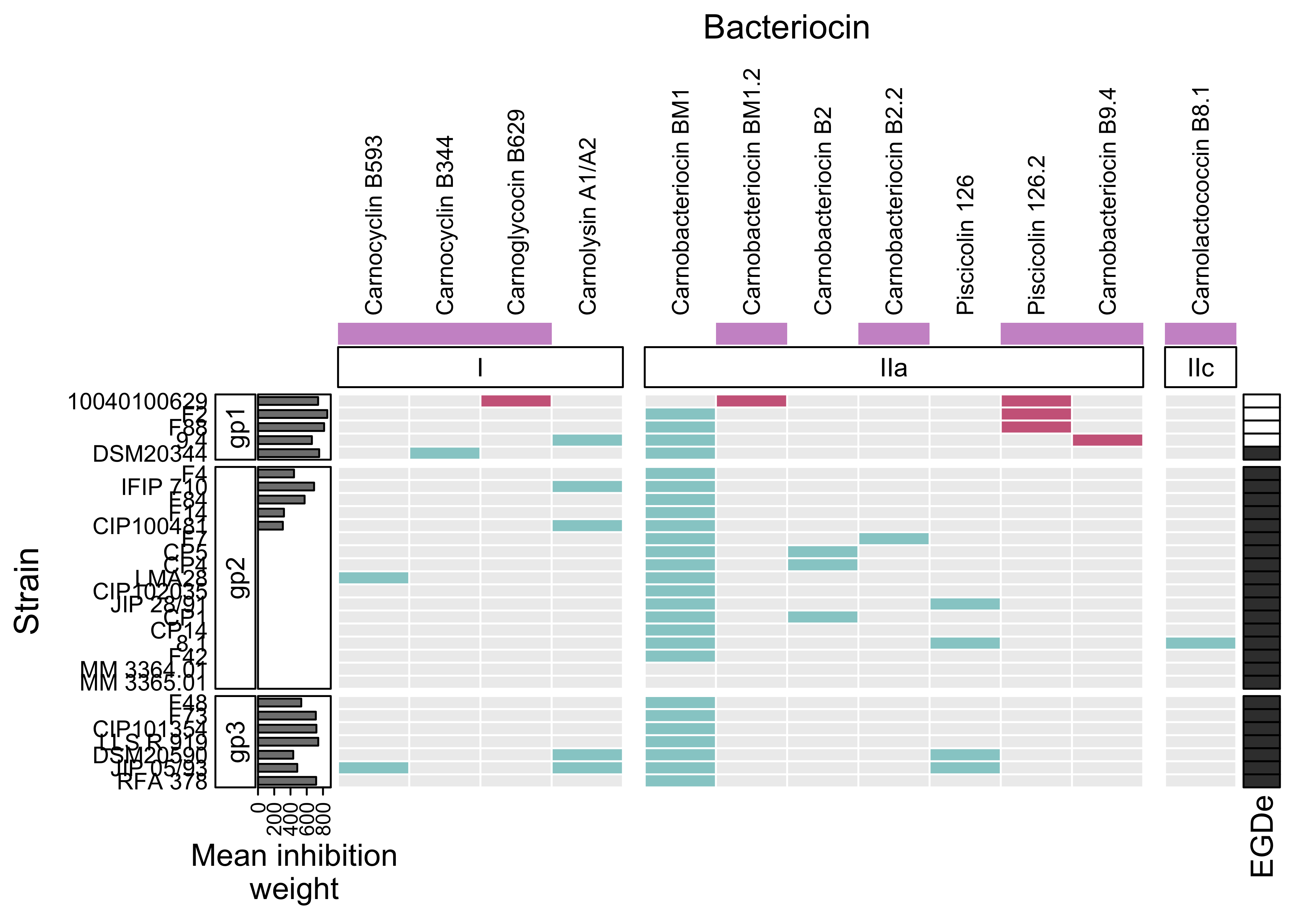
OCCURENCE
DATA PREPARATION
occ <- read.csv2(file = file.path(path,"occurence3_no_imm2.csv"),check.names = F,header = T, stringsAsFactors = T)

occ <- occ %>%
  arrange(factor(Strains, levels = gp$strains))

bacteriocin_new <-read.csv2(file = file.path(path,"bacteriocin_new.csv"),
    check.names = F,
    header = T,
    stringsAsFactors = T)
bacteriocin_new$new <- as.factor(bacteriocin_new$new)
mat_occ <- as.matrix(occ)
rownames(mat_occ) <- mat_occ[,1]
mat_occ <- mat_occ[,-1]
HEATMAP
# calculate the meanweight of inhibition of receivers for each strain for which the genome was sequenced
weight <- mat
weight <- weight %>%
select("from":"F2") %>%
  pivot_longer(cols="ATCC35586":"F2",
               names_to="to",
               values_to="weight") %>%
  mutate(weight=ifelse(weight<300,NA,weight)) %>%
  filter(from %in% genome_yes) %>%
  group_by(from)%>%
  summarize(mean_weight= mean(weight, na.rm=TRUE))
weight$from <- droplevels(weight$from)
weight <- weight[match(rownames(mat_occ), weight$from),]


# define the colors
colors = structure(
  c("gray93","paleturquoise3", "palevioletred3"),#"seashell"
  names = c(0,1,2)
)
t <-mat_inhib_deg2_genome %>%
  select(strains,EGDe_bin)

colnames(t)[colnames(t) == 'EGDe_bin'] <- 'EGDe'

gp <- left_join(gp,t, by="strains")

ha_EGDe <-  rowAnnotation(EGDe = gp$EGDe,
                          col = list(EGDe = c("0" = "white",
                                              "1" = "gray23")),
                          gp = gpar(col = "black"),
                          show_legend = FALSE#,
                             #show_annotation_name = FALSE
                             )

p <- Heatmap(
  mat_occ,

  # NO LEGENDS
  show_heatmap_legend = FALSE,

  # TITLES
  column_title = "Bacteriocin",
  row_title = "Strain",

  # Add frame to each cells
  rect_gp = gpar(col = "white", lwd = 1),
  # Text size for row names
  row_names_gp = gpar(fontsize = 9),
  # Text size for column names
  column_names_gp = gpar(fontsize = 9),

  # names of the rows on the left
  row_names_side = "left",
  column_names_side = "top",
  col = colors,


  # SPLIT COLUMNS
  column_split = c(
    rep("class I", 4),
    rep("Class IIa", 7),
    rep("class IIc", 1)
  ),
  column_gap = unit(3, "mm"),


  # TOP ANNOTATION
  top_annotation = HeatmapAnnotation(
    new  = bacteriocin_new$new,
    col=list(new = c("0" = "white", "1" = "plum3")), #"seagreen3"
    simple_anno_size = unit(0.3,"cm"),
    show_legend = FALSE,
    show_annotation_name = FALSE,
    foo = anno_block(
      gp = gpar(fill = 0:0),
      height = unit(0.55, "cm"),
      labels = c("I", "IIa", "IIc"),
      labels_gp = gpar(col = "black",
                       fontsize = 10),
      )

    ),
  column_km = 3,
  row_split = gp$gp,

  # LEFT ANNOTATION
  left_annotation = rowAnnotation(foo = anno_block(gp = gpar(fill = 0:0),
                                                   labels = c("gp1", "gp2", "gp3"),
                                                   width = unit(0.55, "cm"),
                                                   labels_gp = gpar(col = "black", fontsize = 10)),
                                  "Mean inhibition\nweight"=anno_barplot(weight$mean_weight,
                                                                           width = unit(1,"cm"))),

  row_km = 3,

  # RIGHT ANNOTATION
  right_annotation = ha_EGDe
)
p
rm(p)
REFERENCES
sessionInfo()
## R version 4.2.2 (2022-10-31)
## Platform: aarch64-apple-darwin20 (64-bit)
## Running under: macOS Ventura 13.2.1
##
## Matrix products: default
## BLAS:   /Library/Frameworks/R.framework/Versions/4.2-arm64/Resources/lib/libRblas.0.dylib
## LAPACK: /Library/Frameworks/R.framework/Versions/4.2-arm64/Resources/lib/libRlapack.dylib
##
## locale:
## [1] en_US.UTF-8/en_US.UTF-8/en_US.UTF-8/C/en_US.UTF-8/en_US.UTF-8
##
## attached base packages:
## [1] grid      stats     graphics  grDevices utils     datasets  methods
## [8] base
##
## other attached packages:
##  [1] car_3.1-1             carData_3.0-5         factoextra_1.0.7
##  [4] ggprism_1.0.4         ggthemes_4.2.4        ggrepel_0.9.3
##  [7] viridis_0.6.2         viridisLite_0.4.1     ComplexHeatmap_2.14.0
## [10] lubridate_1.9.2       forcats_1.0.0         stringr_1.5.0
## [13] dplyr_1.1.0           purrr_1.0.1           readr_2.1.4
## [16] tidyr_1.3.0           tibble_3.2.0          ggplot2_3.4.1
## [19] tidyverse_2.0.0
##
## loaded via a namespace (and not attached):
##  [1] nlme_3.1-162        matrixStats_0.63.0  doParallel_1.0.17
##  [4] RColorBrewer_1.1-3  tools_4.2.2         backports_1.4.1
##  [7] bslib_0.4.2         utf8_1.2.3          R6_2.5.1
## [10] BiocGenerics_0.44.0 mgcv_1.8-42         colorspace_2.1-0
## [13] GetoptLong_1.0.5    withr_2.5.0         tidyselect_1.2.0
## [16] gridExtra_2.3       compiler_4.2.2      cli_3.6.0
## [19] labeling_0.4.2      bookdown_0.33       sass_0.4.5
## [22] scales_1.2.1        digest_0.6.31       rmarkdown_2.20
## [25] pkgconfig_2.0.3     htmltools_0.5.4     fastmap_1.1.1
## [28] highr_0.10          rlang_1.0.6         GlobalOptions_0.1.2
## [31] rstudioapi_0.14     shape_1.4.6         jquerylib_0.1.4
## [34] generics_0.1.3      farver_2.1.1        jsonlite_1.8.4
## [37] magrittr_2.0.3      Matrix_1.5-3        Rcpp_1.0.10
## [40] munsell_0.5.0       S4Vectors_0.36.2    fansi_1.0.4
## [43] abind_1.4-5         lifecycle_1.0.3     stringi_1.7.12
## [46] yaml_2.3.7          parallel_4.2.2      crayon_1.5.2
## [49] lattice_0.20-45     splines_4.2.2       circlize_0.4.15
## [52] hms_1.1.2           magick_2.7.3        knitr_1.42
## [55] pillar_1.8.1        ggpubr_0.6.0        rjson_0.2.21
## [58] ggsignif_0.6.4      codetools_0.2-19    stats4_4.2.2
## [61] glue_1.6.2          evaluate_0.20       blogdown_1.16
## [64] png_0.1-8           vctrs_0.5.2         tzdb_0.3.0
## [67] foreach_1.5.2       gtable_0.3.1        clue_0.3-64
## [70] cachem_1.0.7        xfun_0.37           broom_1.0.3
## [73] rstatix_0.7.2       iterators_1.0.14    IRanges_2.32.0
## [76] cluster_2.1.4       timechange_0.2.0    ellipsis_0.3.2